ARTICLE

Optimizing Medium Components for the Maximum Growth of Lactobacillus plantarum JNU 2116 Using Response Surface Methodology

Heeseop Yoo1, Insoo Rheem2, Sungsue Rheem3,*, Sejong Oh4,*
Author Information & Copyright
1JNBIO, Jeonnam 57509, Korea
2Department of Laboratory Medicine, Dankook University Hospital, Cheonan 31116, Korea
3Graduate School of Public Administration, Korea University, Sejong 30019, Korea
4Division of Animal Science, Chonnam National University, Gwangju 61186, Korea
*Corresponding Author : Division of Animal Science, Chonnam National University, Gwangju 61186, Korea Tel: +82-62-530-2116 Fax: +82-62-530-2129 E-mail: soh@jnu.ac.kr
*Corresponding Author : Graduate School of Public Administration, Korea University, Sejong 30019, Korea Tel: +82-44-860-1554 Fax: +82-44-860-1551 E-mail: rheem@korea.ac.kr

© Copyright 2018 Korean Society for Food Science of Animal Resources. This is an Open-Access article distributed under the terms of the Creative Commons Attribution Non-Commercial License (http://creativecommons.org/licenses/by-nc/3.0/) which permits unrestricted non-commercial use, distribution, and reproduction in any medium, provided the original work is properly cited.

Received: Jan 24, 2018 ; Revised: Jan 30, 2018 ; Accepted: Jan 31, 2018

Published Online: Apr 30, 2018

Abstract

This study was undertaken to find the optimum soy-peptone, glucose, yeast extract, and magnesium sulfate amounts for the maximum growth of Lactobacillus plantarum JNU 2116 and to assess the effects of these medium factors through the use of response surface methodology. A central composite design was used as the experimental design for the allocation of treatment combinations. In the analysis of the experiment, due to a significant lack of fit of the second-order polynomial regression model that was used at first, cubic terms were added to the model, and then two-way interaction terms were deleted from the model since they were found to be all statistically insignificant. A relative comparison among the four factors showed that the growth of L. plantarum JNU 2116 was affected strongly by yeast extract, moderately by glucose and peptone, and slightly by magnesium sulfate. The estimated optimum amounts of the medium factors for the growth of L. plantarum JNU 2116 are as follows: soy-peptone 0.213%, glucose 1.232%, yeast extract 1.97%, and magnesium sulfate 0.08%. These results may contribute to the production of L. plantarum L67 as a starter culture that may have potential application in yogurt and fermented meat products.

Keywords: response surface methodology; optimization; growth; Lactobacillus plantarum

Introduction

Lactobacillus species are the most frequently and safely used probiotics. It is even commonly consumed by children and immunocompromised individuals (Borriello et al., 2003). In particular, Lactobacillus plantarum, a member of the hetero-fermentative group of Lactobacilli, is a heterogeneous and versatile species that is encountered in a variety of environmental niches, including silage, sourdough, fish, and many fermented vegetables (Seddik et al., 2017). Traditionally, L. plantarum was not used in yogurt fermentation, but it was used in fermented sausages and some types of cheese. According to a recent report, L. plantarum L67, which has a high survival rate at low pH, was found to have been mixed with lactic acid bacteria as a starter culture and could be used for making yogurt (Song et al., 2016).

The species of L. plantarum exhibits various biological effects, including antitumor, anticoagulant, antiviral, immunomodulatory, anti-inflammatory, antidiabetic, antioxidative, and free radical-scavenging activities (Andersson et al., 2010; Giardina et al., 2014).

In a previous study (Jeong et al., 2015), we determined that L. plantarum JNU 2116, isolated from kimchi, has a high survival rate at low pH. Strain JNU 2116 produces an anticarcinogenic peptide (NH2-XLEXKKAEXITTXX) in the presence of mutagens (4-nitroquinoline 1-oxide, N-methyl-N'-nitro-N-nitrosoguanidine, and 2-amino-3-methylimidazole quinoline).

The growth of lactic acid bacteria is greatly affected by the fermentation conditions, such as temperature, pH, medium components, and oxygen, among which the types of growth medium play an important role in bacterial viability. For growing lactic acid bacteria, MRS and M17 media, as well as skim milk, are used extensively. Tryptone, a medium component produced by the digestion of milk caseins by trypsin (Fraser and Powell, 1950), provides an excellent source of amino acids and small peptides for growing microorganisms and is therefore commonly incorporated into the growth media of lactic acid bacteria and other microorganisms.

In order to use probiotics as a health supplement, the fermentation process is a critical factor in large-scale production for enhancing the cell yield (Maÿyra-Mäkinen and Bigret, 1993). Thus, the evaluation of the medium ingredients should be carried out for fermentation optimization. Oh et al. (1995) suggested that a modified response surface (RS) model with cubic and quartic terms could find a more optimal point and thus could assess factor effects more appropriately.

In this study, using a new RS modeling approach, we evaluated the effects of the four medium components that are soy-peptone, glucose, yeast extract, and magnesium sulfate, and estimated the optimum growth conditions for enhancing viable cells of L. plantarum JNU 2116.

Materials and Methods

Experimental design

A central composite design (Myers et al., 2009) in 6 blocks was used to allocate treatment combinations in this experiment, which consisted of 36 runs and was conducted for 6 days (Table 1). Each of the first 4 blocks, which represented days 1, 2, 3, and 4 of the experiment, contained 4 factorial runs and 2 center runs. Each of the last 2 blocks, which represented days 5 and 6 of the experiment, contained 4 axial runs and 2 center runs.

Table 1. Treatment combinations and responses
No. Block Peptone Glucose Yeast extract Magnesium sulfate OD Log (CFU)
(g/L) [×1] (g/L) [×2] (g/L) [×3] (g/L) [×4]
1 0 1 [–1] 7 [–1] 5 [–1] 0.5 [–1] 1.532 8.72098574
2 0 3 [ 1] 7 [–1] 5 [–1] 0.5 [–1] 1.328 8.98944982
3 0 1 [–1] 21 [ 1] 5 [–1] 0.5 [–1] 1.171 8.6127839
4 0 3 [ 1] 21 [ 1] 5 [–1] 0.5 [–1] 1.33 8.61278386
5 0 2 [ 0] 14 [ 0] 10 [ 0] 1 [ 0] 1.577 8.979093
6 0 2 [ 0] 14 [ 0] 10 [ 0] 1 [ 0] 1.589 8.960471
7 1 1 [–1] 7 [–1] 15 [ 1] 0.5 [–1] 1.741 8.90471554
8 1 3 [ 1] 7 [–1] 15 [ 1] 0.5 [–1] 1.714 8.95760729
9 1 1 [–1] 21 [ 1] 15 [ 1] 0.5 [–1] 1.666 8.9444827
10 1 3 [ 1] 21 [ 1] 15 [ 1] 0.5 [–1] 1.695 8.89762709
11 1 2 [ 0] 14 [ 0] 10 [ 0] 1 [ 0] 1.524 8.829947
12 1 2 [ 0] 14 [ 0] 10 [ 0] 1 [ 0] 1.548 8.85309
13 2 1 [–1] 7 [–1] 5 [–1] 1.5 [ 1] 1.166 8.63346845
14 2 3 [ 1] 7 [–1] 5 [–1] 1.5 [ 1] 1.293 8.63346846
15 2 1 [–1] 21 [ 1] 5 [–1] 1.5 [ 1] 1.14 8.6263404
16 2 3 [ 1] 21 [ 1] 5 [–1] 1.5 [ 1] 1.322 8.69722934
17 2 2 [ 0] 14 [ 0] 10 [ 0] 1 [ 0] 1.554 8.878522
18 2 2 [ 0] 14 [ 0] 10 [ 0] 1 [ 0] 1.566 8.860937
19 3 1 [–1] 7 [–1] 15 [ 1] 1.5 [ 1] 1.723 8.85491302
20 3 3 [ 1] 7 [–1] 15 [ 1] 1.5 [ 1] 1.763 8.99694925
21 3 1 [–1] 21 [ 1] 15 [ 1] 1.5 [ 1] 1.678 8.8481891
22 3 3 [ 1] 21 [ 1] 15 [ 1] 1.5 [ 1] 1.684 8.88817949
23 3 2 [ 0] 14 [ 0] 10 [ 0] 1 [ 0] 1.457 8.90309
24 3 2 [ 0] 14 [ 0] 10 [ 0] 1 [ 0] 1.506 8.742725
25 4 0 [–2] 14 [ 0] 10 [ 0] 1 [ 0] 1.101 8.42488163
26 4 4 [ 2] 14 [ 0] 10 [ 0] 1 [ 0] 1.531 8.53529412
27 4 2 [ 0] 0 [–2] 10 [ 0] 1 [ 0] 0.701 8.3283796
28 4 2 [ 0] 28 [ 2] 10 [ 0] 1 [ 0] 1.433 8.64443859
29 4 2 [ 0] 14 [ 0] 10 [ 0] 1 [ 0] 1.423 8.740363
30 4 2 [ 0] 14 [ 0] 10 [ 0] 1 [ 0] 1.427 8.799341
31 5 2 [ 0] 14 [ 0] 0 [–2] 1 [ 0] 0.409 8.23299611
32 5 2 [ 0] 14 [ 0] 20 [ 2] 1 [ 0] 1.905 9.14921911
33 5 2 [ 0] 14 [ 0] 10 [ 0] 0 [–2] 1.409 8.8802418
34 5 2 [ 0] 14 [ 0] 10 [ 0] 2 [ 2] 1.722 9.071882
35 5 2 [ 0] 14 [ 0] 10 [ 0] 1 [ 0] 1.591 8.888179
36 5 2 [ 0] 14 [ 0] 10 [ 0] 1 [ 0] 1.596 8.857332
Download Excel Table

In this experiment, the response, Log (CFU), was assumed to be under the influence of the 4 medium factors mentioned in the Introduction. To set up a statistical model, we denoted Log (CFU) by Y and determined the coded factor levels as follows:

X1=(peptone–2)/1, X2=(glucose–14)/7, X3=(yeast extract–10)/5, and X4=(magnesium sulfate–1)/0.5.

Table 2 contains the actual factor levels corresponding to the coded factor levels. The observed responses of the treatment combinations are presented in Table 1. Using this design, we could fit a second- or higher-order polynomial regression model to the data.

Table 2. Actual factor levels corresponding to the coded factor levels
Actual factor Coded factor Actual factor level at the coded factor level of
–2 –1 0 1 2
Peptone (g/L) X1 0 1 2 3 4
Glucose (g/L) X2 0 7 14 21 28
Yeast extract (g/L) X3 0 5 10 15 20
Magnesium sulfate (g/L) X4 0 0.5 1 1.5 2
Download Excel Table
Bacterial strain and the enumeration of viable cells

L. plantarum JNU 2116 was obtained from stock cultures maintained by the Dairy Microbiology Laboratory at Chonnam National University (Gwangju, Korea). L. plantarum JNU 2116 was grown for overnight at 37°C in de Man Rogosa Sharpe broth (1960; MRS) and was subcultured three times prior to use. Stock culture of L. plantarum JNU 2116 was stored at -80°C in 10% (v/v) skim milk containing cryoprotectant. For the enumeration of L. planatrum JNU2116, the appropriate diluted-samples were plated by using MRS agar. The plates were incubated at 37°C for 48 h.

Statistical analysis

Data were analyzed using SAS software (SAS Korea, SAS® 9.4). SAS/STAT (2013) procedures were used for regression modeling. Optimum conditions were found through SAS data-step programming. The plots were generated by SAS/GRAPH (2013).

Results and Discussion

Developing a regression model

First, the second-order polynomial regression model containing 4 linear, 4 quadratic, and 6 interaction terms plus 5 dummy variables for 6 blocks was employed by using the RSREG procedure of SAS/STAT. The analysis of variance for evaluation of the second-order model is presented in Table 3.

Table 3. Analysis of variance for evaluation of the second-order model
Regression Degrees of freedom Type I sum of squares r2 F-value p-value
Covariates 5 0.42846 0.3054 7.94 0.0006
Linear 4 0.56331 0.4016 13.04 <0.0001
Quadratic 4 0.20883 0.1489 4.84 0.0095
Interactions 6 0.02942 0.0210 0.45 0.8318
Total model 19 1.23002 0.8768 6.00 0.0004
Residual Degrees of freedom Sum of squares Mean square F-value p-value
Lack of fit 10 0.15710 0.01571 6.02 0.0197
Pure error 6 0.01567 0.00261
Total error 16 0.17276 0.01080
Download Excel Table

Table 3 shows that the r2 value of the second-order model was 0.8768 and the lack of fit was significant (p=0.0197). This suggested that this regression model did not accurately represent the data in the experimental region, indicating that cubic terms might have to be included in the model. Thus, a third-order polynomial model containing 4 linear, 4 quadratic, 4 cubic, and 6 interaction terms plus 5 dummy variables for 6 blocks was fitted to the data. Table 4 displays the analysis of variance for this third-order model.

Table 4. Analysis of variance for evaluation of the third-order model
Regression Degrees of freedom Type I sum of squares r2 F-value p-value
Covariates 5 0.42846 0.3054 13.20 0.0002
Linear 4 0.56331 0.4016 21.69 <0.0001
Quadratic 4 0.20883 0.1489 8.04 0.0022
Cubic 4 0.09484 0.0676 3.65 0.0362
Interactions 6 0.02942 0.0210 0.75 0.6179
Total model 23 1.32486 0.9444 8.87 0.0002
Residual Degrees of freedom Sum of squares Mean square F-value p-value
Lack of fit 6 0.06226 0.01038 3.97 0.0587
Pure error 6 0.01567 0.00261
Total error 12 0.07793 0.00649
Download Excel Table

As shown in Table 4, the r2 value of this third-order model was 0.9444, the lack of fit of the model was barely insignificant (p=0.0587) at the 5% level, and interactions were not significant with an F-value less than 1 (p=0.6179). Thus, in anticipation of an improvement of the model, we got rid of the interaction trms in Table 4. Table 5 shows the analysis of variance of this third-order model without interaction terms.

Table 5. Analysis of variance for evaluation of the reduced third-order model
Regression Degrees of freedom Type I sum of squares r2 F-value p-value
Covariates 5 0.42846 0.3054 14.37 <0.0001
Linear 4 0.56331 0.4016 23.61 <0.0001
Quadratic 4 0.20883 0.1489 8.75 0.0004
Cubic 4 0.09484 0.0676 3.98 0.0175
Total model 17 1.29544 0.9235 12.78 <0.0001
Residual Degrees of freedom Sum of squares Mean square F-value p-value
Lack of fit 12 0.09168 0.00764 2.93 0.0985
Pure error 6 0.01567 0.00261
Total error 18 0.10734 0.00596
Download Excel Table

From Table 5, we see that the r2 value of this reduced third-order model was 0.9235, the lack of fit of this model was more insignificant (p=0.0985), and each of the covariate, linear, quadratic, and cubic parts contained at least one significant term. This model had fewer terms than the full second-order model in Table 3, yet it produced a larger r2 value and an insignificant lack of fit. Thus, we used this model as the final one for the medium optimization. The coefficients are given in Table 6, where D1, D2, D3, D4, and D5 were defined as follows: if day=1, then D1=1, D2=0, D3=0, D4=0, D5=0; if day=2, then D1=0, D2=1, D3=0, D4=0, D5=0; if day=3, then D1=0, D2=0, D3=1, D4=0, D5=0; if day=4, then D1=0, D2=0, D3=0, D4=1, D5=0; if day=5, then D1=0, D2=0, D3=0, D4=0, D5=1; and if day=6, then D1=0, D2=0, D3=0, D4=0, D5=0.

Table 6. Coefficient estimates from the third-order model without interactions
Variable Parameter estimate Standard error t-value p-value
Intercept b0=8.83360 0.04816 183.43 <0.0001
D1 a1=0.15174 0.06305 2.41 0.0271
D2 a2=0.03152 0.06305 0.5 0.6232
D3 a3=0.05973 0.06305 0.95 0.356
D4 a4=0.00487 0.06305 0.08 0.9393
D5 a5=–0.10291 0.07722 –1.33 0.1993
X1 b1=0.03475 0.02730 1.27 0.2193
X12 b11=–0.05776 0.01672 –3.45 0.0028
X13 b111=–0.00179 0.01115 –0.16 0.8744
X2 b2=–0.07333 0.02730 –2.69 0.0151
X22 b22=–0.05618 0.01672 –3.36 0.0035
X23 b222=0.03809 0.01115 3.42 0.0031
X3 b3=0.12919 0.04550 2.84 0.0109
X32 b33=–0.03073 0.01672 –1.84 0.0826
X33 b333=0.02497 0.01439 1.74 0.0998
X4 b4=–0.01489 0.04550 –0.33 0.7472
X42 b44=0.04051 0.01672 2.42 0.0262
X43 b444=0.01570 0.01439 1.09 0.2896
Download Excel Table
Comparing the third-order polynomial effects of the factors

Our response surface model is written as

Ŷ= b0+a1 D1+a2 D2+a3 D3+a4 D4+a5 D5+f̂ (X1)+f̂ (X2)+f̂ (X3)+f̂ (X4)
where
f̂ (Xj)=bj Xj+bjj Xj2+bjjj Xj3, j=1, 2, 3, 4

In the equation, Ŷ denotes the predicted value of Y, and for j=1, 2, 3, 4, each f̂ (Xj) denotes an estimate of the original function f(Xj)=βj Xjjj Xj2jjj Xj3.

For k≧2, a kth-order polynomial effect of the factor Xj is defined as the F-value in testing if all the coefficients of the linear term, the quadratic term, …, and the kth-power term of Xj are zero. To compare the third-order polynomial effects of the factors X1, X2, X3, and X4, we compared the F-values and p-values from testing.

Ho: βjjjjjj=0, j=1, 2, 3, 4.

Table 7 contains the results from these tests.

From Table 7, we can see that the F-value for X3 (yeast extract) was the largest (31.67), those for X2 (glucose) and X1 (peptone) were similar in the middle group (7.67 and 5.29, respectively), and that for X4 (magnesium sulfate) was the smallest (2.98). Thus, in relative comparison, the order of the factors according to the magnitude of the third-order polynomial effect is as follows:

Table 7. Test results from comparison of the third-order polynomial effects of the factors
Result from testing Ho: β111111=0 (Factor: Peptone)
Source Degrees of freedom Mean square F-value p-value
Numerator 3 0.03155 5.29 0.0086
Denominator 18 0.00596
Result from testing Ho: β222222=0 (Factor: Glucose)
Source Degrees of freedom Mean square F-value p-value
Numerator 3 0.04572 7.67 0.0017
Denominator 18 0.00596
Result from testing Ho: β333333=0 (Factor: Yeast extract)
Source Degrees of freedom Mean square F-value p-value
Numerator 3 0.18887 31.67 <0.0001
Denominator 18 0.00596
Result from testing Ho: β444444=0 (Factor: Magnesium sulfate)
Source Degrees of freedom Mean square F-value p-value
Numerator 3 0.01779 2.98 0.0587
Denominator 18 0.00596

yeast extract>glucose≅peptone>magnesium sulfate.

Download Excel Table
Drawing the third-order polynomial effect plots of the factors

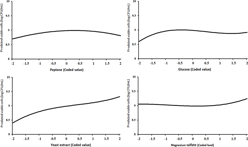
Since there were no interaction terms in the final model, we could draw the third-order polynomial effect plots of each factor separately (Fig. 1).
kosfa-38-2-240-g1
Fig. 1. Third-order polynomial effect plots of peptone, glucose, yeast extract, and magnesium sulfate in the range of –2 to 2 (in coded level), from left to right.
Download Original Figure

In Fig. 1, the 4 plots depict f̂ (Xj)=bj Xj+bjj Xj2+bjjj Xj3, j=1, 2, 3, 4, respectively, from left to right. The values of bj, bjj, and bjjj, j=1, 2, 3, 4, are given in Table 6. The shapes of these 4 curves were in accordance with the 4 test results in Table 7.

A relative comparison using Fig. 1 also says that the growth of L. plantarum JNU 2116 was affected strongly by yeast extract, moderately by glucose and peptone, and slightly by magnesium sulfate.

Finding the optimum point of the factors

Through a search on a grid (Oh et el., 1995), we maximized the predicted response from the model with the coefficients in Table 6, assuming that the values of the block variables were D1=1, D2=0, D3=0, D4=0, and D5=0. The bounds for the factor levels were –2≦Xj≦2, j=1, 2, 3, 4, and the radius of the spherical region of the experimental design displayed in Table 1 was 2. Thus, with the bounds of –2≦Xj≦2, j=1, 2, 3, 4, we made a search within the spherical region with the radius of 2, for which the constraint was X12+X22+X32+X42≦22=4. This search, which was conducted using SAS data-step programming, determined the optimum point, described in Table 8.

Table 8. Optimization results from an exploration within the hypersphere with a radius of 2
X1 X2 X3 X4 Distance from the origin Predicted maximum Log(CFU) Peptone (g/L) Glucose (g/L) Yeast extract (g/L) Magnesium sulfate (g/L)
0.13 –0.24 1.94 –0.4 1.9995 9.3314 2.31 12.32 19.7 0.8
Download Excel Table
Experimenting for validation

A validation experiment was performed to verify the optimization results in Table 8. Table 9 shows the medium composition from the optimization results, which was used for the validation experiment.

Table 9. Optimum medium composition and the results of the validation experiment
Component (%) MRS medium Optimum medium
Soy peptone - 0.231
Proteose peptone 1.0 -
Glucose 2.0 1.232
Yeast extract 0.5 1.97
Magnesium sulfate 0.01 0.08
Ammonium citrate 0.2 -
Beef extract 1.0 -
Manganese sulfate 0.005 -
Potassium phosphate dibasic 0.2 -
Sodium acetate 0.5 -
Tween 80 0.1 -
Viable cells (Log CFU/mL) 9.51 9.15

a absence of constituent.

Download Excel Table

To verify the validity of the optimum medium with the composition in Table 9, our validation experiment compared it with MRS broth, a frequently used commercial medium.

The data in Table 9 show that for both media, the number of viable cells was more than 109 (CFU/mL), which is a good result. Our optimum medium turned out to be economically viable in that the price for producing as much as 300 liters of it is as cheap as a little over 100 US dollars, and its cultivation amount is as much as 96.2% that of MRS broth.

Drawing 3D response surface plots

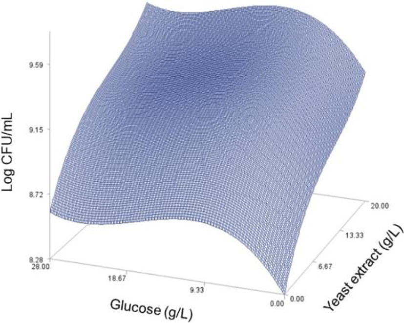
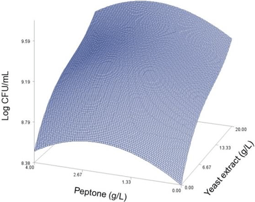
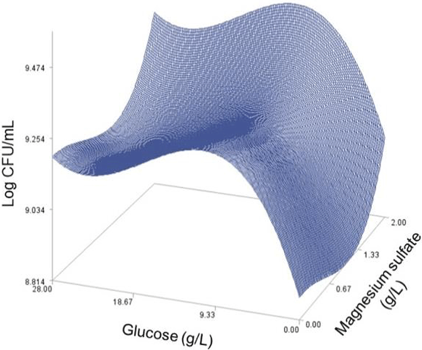
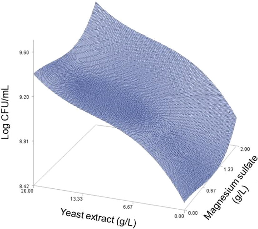
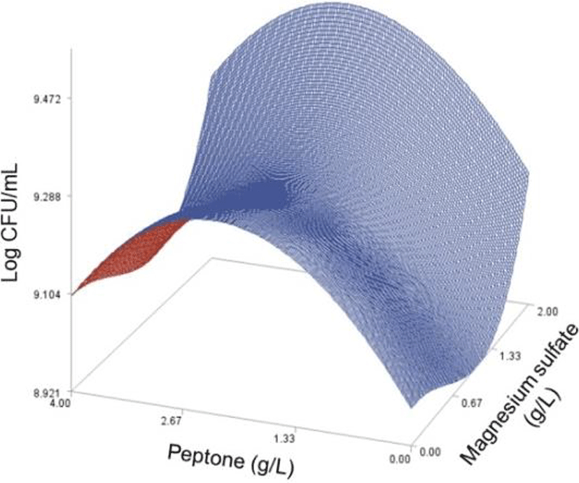
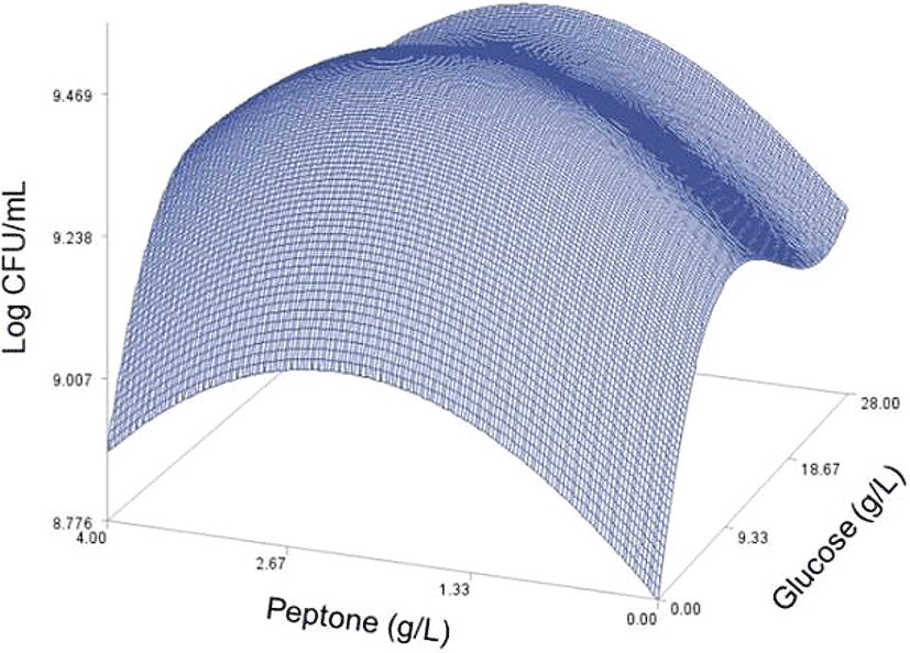
As done in the paper by Oh et el. (1995), for any 2 of the 4 factors, a three-dimensional response surface plot was drawn, with the vertical axis representing the predicted viable cells (Log CFU) and the 2 horizontal axes representing the actual levels of 2 explanatory factors. In these plots, the values of the block variables were set to be D1=1, D2=0, D3=0, D4=0, and D5=0.

In each plot, the factors not represented by the 2 horizontal axes are fixed at their optimum actual levels. From all 6 plots produced (Figs 2 through 7), we can see that the effects of the pairs of the factors were additive since there were no interactions. By the additivity of the 2-factor effects, we mean that the effect of one factor on the response does not depend on the level of the other factors (Oh et al., 1995).
kosfa-38-2-240-g4
Fig. 2. Response surface plot for the effects of peptone and glucose on the predicted viable cells at yeast extract=17.5 (g/L) and magnesium sulfate=1.99 (g/L).
Download Original Figure
kosfa-38-2-240-g2
Fig. 3. Response surface plot for the effects of peptone and yeast extract on the predicted viable cells at glucose=12.25 (g/L) and magnesium sulfate=1.99 (g/L).
Download Original Figure
kosfa-38-2-240-g5
Fig. 4. Response surface plot for the effects of peptone and magnesium sulfate on the predicted viable cells at glucose=12.25 (g/L) and yeast extract=17.5 (g/L).
Download Original Figure
kosfa-38-2-240-g3
Fig. 5. Response surface plot for the effects of glucose and yeast extract on the predicted viable cells at peptone=2.13 (g/L) and magnesium sulfate=1.99 (g/L).
Download Original Figure
kosfa-38-2-240-g6
Fig. 6. Response surface plot for the effects of glucose and magnesium sulfate on the predicted viable cells at peptone=2.13 (g/L) and yeast extract=17.5 (g/L).
Download Original Figure
kosfa-38-2-240-g7
Fig. 7. Response surface plot for the effects of yeast extract and magnesium sulfate on the predicted viable cells at peptone=2.13 (g/L) and glucose=12.25 (g/L).
Download Original Figure

Conclusion

Using a new response surface approach, we developed a statistical model to assess the third-order polynomial effects of the four medium components on the growth of L. plantarum JNU 2116, and established their estimated optimum levels to maximize its growth, which are soy-peptone 0.213%, glucose 1.232%, yeast extract 1.97%, and magnesium sulfate 0.08%, through a validation experiment. Our optimum medium turned out to be economically viable in that its production price is cheaper than that of MRS broth and its cultivation amount is close to that of MRS broth.


Acknowledgements

This study was support by the Jeollannam-do (2016 R & D supporting program operated by Jeonnam Technopark) and by a Korea University Grant.

References

1.

Andersson U, Bränning C, Ahrné S, Molin G, Alenfall J, Onning G, Nyman M, Holm C. Probiotics lower plasma glucose in the high-fat fed C57BL/6J mouse. Benef Microbes. 2010; 1:189-196.

2.

Borriello SP, Hammoles WP, Holzapfel W, Marteau P, Schrezenmeir J, Vaara M, Valtenen V. Safety of probiotics that contain Lactobacilli or Bifidobacteria. Clin Infect Dis. 2003; 36:775-780.

3.

De Man JC, Rogosa M, Sharpe ME. A medium for the cultivation of Lactobacilli.. J Appl Microbiol. 1960; 23:130-135.

4.

Giardina S, Scilironi C, Michelotti A, Samuele A, Borella F, Daglia M, Marzatico F. In vitro anti-inflammatory activity of selected oxalate-degrading probiotic bacteria: Potential applications in the prevention and treatment of hyperoxaluria. J Food Sci. 2014; 79:384-390.

5.

Fraser D, Powell RE. The kinetics of trypsin digestion. J Biol Chem. 1950; 187:803-820.

6.

Jeong JU, Song M, Kim Y, Kim KH, Kang J, Oh S. Characterisation and partial purification of an antimutagenic peptide produced by Lactobacillus plantarum JNU 2116. Int J Dairy Technol. 2015; 68:582-588.

7.

Maÿyra-Mäkinen A, Bigret N. Industrial use and production of lactic acid bacteria. Lactic acid bacteria. In: Salminen A, von Wright A, editors.Marcel Dekker Inc. New York, USA: p. 65-95.

8.

Myers RH, Montgomery DC, Anderson-Cook CM. Response surface methodology: Process and product optimization using designed experiments. 3rd ed.Wiley. UK: .

9.

Oh S. Probiotics in dairy products. Beneficial microorganisms in food and nutraceuticals. In: Liong MT, editor.Springer International Publishing. Switzerland: p. 203-219.

10.

Oh S, Rheem S, Sim J, Kim S, Baek Y. Optimizing conditions for the growth of Lactobacillus casei YIT 9018 in tryptone-glucose medium by using response surface methodology. Appl Environ Microbiol. 1995; 61:3809-3814.

11.

SAS Institute Inc SAS/STAT user’s guide, release 6.04. SAS Institute Inc. Cary, NC, USA: .

12.

Seddik HA, Bendali F, Gancel F, Fliss I, Spano G, Drider D. Lactobacillus plantarum and its probiotic and food potentialities. Probiotics Antimicrob Proteins. 2017; 9:111-122.

13.

Song S, Lee SJ, Park DJ, Oh S, Lim KT. The anti-allergic activity of Lactobacillus plantarum L67 and its application to yogurt. J Dairy Sci. 2016; 99:9372-9382.