Improving the Quality of Response Surface Analysis of an Experiment for Coffee-supplemented Milk Beverage: II. Heterogeneous Third-order Models and Multi-response Optimization

Rheem, Sungsue; Rheem, Insoo; Oh, Sejong

doi:10.5851/kosfa.2019.e17

Food Sci Anim Resour 2019; 39(2):222-228

pISSN: 2636-0772, eISSN: 2636-0780

DOI: https://doi.org/10.5851/kosfa.2019.e17

ARTICLE

Improving the Quality of Response Surface Analysis of an Experiment for Coffee-supplemented Milk Beverage: II. Heterogeneous Third-order Models and Multi-response Optimization

Sungsue Rheem¹^,^*

, Insoo Rheem²

, Sejong Oh³^,^*

Author Information & Copyright ▼

¹Graduate School of Public Administration, Korea University, Sejong 30019, Korea

²Department of Laboratory Medicine, Dankook University Hospital, Cheonan 31116, Korea

³Division of Animal Science, Chonnam National University, Gwangju 61186, Korea

^*Corresponding author : Sungsue Rheem, Graduate School of Public Administration, Korea University, Sejong 30019, Korea Tel: +82-10-8725-7124, E-mail: rheem@korea.ac.kr

^*Corresponding author : Sejong Oh, Division of Animal Science, Chonnam National University, Gwangju 61186, Korea Tel: +82-62-530-2116, E-mail: soh@jnu.ac.kr

© Korean Society for Food Science of Animal Resources. This is an Open-Access article distributed under the terms of the Creative Commons Attribution Non-Commercial License (http://creativecommons.org/licenses/by-nc/3.0) which permits unrestricted non-commercial use, distribution, and reproduction in any medium, provided the original work is properly cited.

Received: Feb 11, 2019 ; Revised: Feb 21, 2019 ; Accepted: Feb 22, 2019

Published Online: Apr 30, 2019

Abstract

This research was motivated by our encounter with the situation where an optimization was done based on statistically non-significant models having poor fits. Such a situation took place in a research to optimize manufacturing conditions for improving storage stability of coffee-supplemented milk beverage by using response surface methodology, where two responses are Y₁=particle size and Y₂=zeta-potential, two factors are F₁=speed of primary homogenization (rpm) and F₂=concentration of emulsifier (%), and the optimization objective is to simultaneously minimize Y₁ and maximize Y₂. For response surface analysis, practically, the second-order polynomial model is almost solely used. But, there exists the cases in which the second-order model fails to provide a good fit, to which remedies are seldom known to researchers. Thus, as an alternative to a failed second-order model, we present the heterogeneous third-order model, which can be used when the experimental plan is a two-factor central composite design having -1, 0, and 1 as the coded levels of factors. And, for multi-response optimization, we suggest a modified desirability function technique. Using these two methods, we have obtained statistical models with improved fits and multi-response optimization results with the predictions better than those in the previous research. Our predicted optimum combination of conditions is (F₁, F₂)=(5,000, 0.295), which is different from the previous combination. This research is expected to help improve the quality of response surface analysis in experimental sciences including food science of animal resources.

Keywords: response surface methodology; central composite design; heterogeneous third-order model; multi-response optimization; desirability

Introduction

Response surface methodology (RSM) is a set of statistical techniques for modeling and optimizing responses through the design and analysis of experiments (Myers et al., 2009), which has been widely used in engineering, agriculture, life science, microbiology and food sciences. A search by Google Scholar revealed that the number of scientific articles whose titles mentioned ‘response surface’ was 157 in 2000 but it became 1,860 in 2018, which is an 11.8-fold increase during recent 18 years. This indicates that RSM has been established as an important tool for modeling and optimization in experimental sciences including food sciences of animal resources.

In RSM, the central composite designs (CCD, Box and Wilson, 1951) have been most frequently used as experimental plans, and the second-order polynomial regression models have been usually employed for data analysis. And, the response surface model can be said to be well fitted and reliable when it satisfies the following criteria: (1) the model is significant (the model p-value≦0.05), (2) the lack of fit is non-significant (the lack-of-fit p-value>0.05), (3) the r²≧0.9 (Giunta, 1997), and (4) the adjusted r²≧0.8 (Myers et al., 2009).

However, in reality, it is observed that, for some data, the analysis models, which are the second-order models in most cases, do not satisfy the above criteria. A remedy in this case is to use a third-order model that consists of linear, quadratic, cubic, and relevant interaction terms (Rheem and Rheem, 2012). For example, when there are two factors, letting X₁ and X₂ denote coded factors, the third-order model has the following terms: linear terms X₁ and X₂, quadratic terms X₁² and X₂², cubic terms X₁³ and X₂³, and the two-factor interaction term X₁X₂. There exist the cases where this method improves the model. But, this method is applicable to a CCD that uses five values, which are denoted by −α, −1, 0, 1, and α, as the levels of coded factors.

When the experimental design is a CCD in which −1, 0, and 1 are the levels of coded factors, as in Table 1, cubic terms cannot be added to the model, since (−1)³=−1, (0)³=0, and (1)³=1, which makes the cubic terms equal to the linear terms. For example, in Table 1B, we can see that X₁=X₁³ and X₂=X₂³, and thus the X₁³ and X₂³ terms cannot be chosen from among the candidates of additional model terms for augmenting the second-order model.

Table 1. Response variables, actual and coded factors, experimental design, and response data

A. Response variables, actual and coded factors, and the levels of the factors
Response variables	Actual factors	Coded factors	Actual factor level corresponding to the coded factor level of
Response variables	Actual factors	Coded factors	−1	0	1
Y₁=Particle size	F₁=Speed of primary homogenization (rpm)	X₁	5,000	10,000	15,000
Y₂=Zeta-potential	F₂=Concentration of emulsifier (%)	X₂	0.1	0.2	0.3

B. Experimental design and response data with candidates of additional model terms
Experimental design in coded levels and response data						Candidates of additional model terms for augmenting the 2^nd-order model
Standard order	Design point	X₁	X₂	Y₁	Y₂	X₁³	X₂³	X₁²X₂	X₁X₂²
1	1	−1	−1	179.900	27.5000	−1	−1	−1	−1
2	2	−1	1	178.267	29.9667	−1	1	1	−1
3	3	1	−1	179.533	24.3000	1	−1	−1	1
4	4	1	1	219.767	32.5666	1	1	1	1
5	5	−1	0	217.867	36.1000	−1	0	0	0
6	6	1	0	178.367	28.2667	1	0	0	0
7	7	0	−1	185.333	29.1000	0	−1	0	0
8	8	0	1	182.167	28.2000	0	1	0	0
9	9	0	0	186.433	30.8300	0	0	0	0
10	9	0	0	181.933	29.0667	0	0	0	0
11	9	0	0	175.633	29.6000	0	0	0	0
12	9	0	0	180.333	29.1000	0	0	0	0

Download Excel Table Download Excel Table

This problem can be solved by adding the terms of the interaction between the linear term of one factor and the quadratic term of another factor. For example, in Table 1B, X₁²X₂ and X₁X₂² are such interaction terms. The model that contains such interaction terms can be named a heterogeneous third-order model, since the sum of the exponents in each of such interaction terms is three. Thus, a remedy in this case is to augment the second-order model to the heterogeneous third-order model by adding the X₁²X₂ and X₁X₂² terms, which are chosen from among the candidates of additional model terms in Table 1B, to the second-order model.

A dataset, which is obtained through the screening of the data in Ahn et al. (2017), will be re-analyzed for the illustration of the remedy suggested in this research note. Since Ahn et al. (2017) has two responses and a purpose of it is the multi-response optimization of them, this research note, which is a continuation of Rheem and Oh (2019), will model both responses by using heterogeneous third-order models, and optimize them simultaneously by employing the desirability function technique.

Materials and Methods

Dataset to be re-analyzed

Data analysis should include data screening, which is necessary for accurate modeling. The original data to be used for re-analysis is the data described in Ahn et al. (2017), in which they tried to optimize manufacturing conditions for improving storage stability of coffee-supplemented milk beverage by using RSM. Through data screening, one outlier was deleted from their data (Rheem and Oh, 2019). The response variables, Y₁ and Y₂, and the factors in this experiment are described in Table 1A. The dataset from which an outlier is eliminated is given in Table 1B. Here, the experimental design is a CCD for two factors with the coded levels of −1, 0, and 1. Using this data, we will fit to the data second-order models and heterogeneous third-order models.

Statistical analysis

Data were analyzed by the use of SAS software. SAS/STAT (2013) was employed for the statistical modeling of data. Graphs were produced by SAS/GRAPH (2013).

Results and Discussion

Fitting the second-order model to the data

First, for each of Y₁ and Y₂, the second-order polynomial regression model containing 2 linear, 2 quadratic, and 1 interaction terms was fitted to the data by using RSREG procedure of SAS/STAT.

For both Y₁ and Y₂, the second-order models are unsatisfactory. For Y₁, the model is non-significant (p=0.5962), the lack of fit is significant (p=0.0131), the r²=0.40<0.9, and the adjusted r²=−0.11<0.8. Also, for Y₂, the model is non-significant (p=0.2924), the lack of fit is significant (p=0.0203), and the r²=0.57<0.9, and the adjusted r²=0.21<0.8. None of the four criteria are met for both Y₁ and Y₂. Thus, we will augment the analysis models for their improvement.

Fitting the heterogeneous third-order model to the data

For each of Y₁ and Y₂, since the second-order model has a poor fit for the data, next we will fit to the data a heterogeneous third-order model that consists of the X₁, X₂, X₁², X₂², X₁X₂, X₁²X₂, and X₁X₂² terms, by adding the X₁²X₂ and X₁X₂² terms to the second-order model, in the anticipation of a possible improvement in modeling.

For both Y₁ and Y₂, the heterogeneous third-order models are satisfactory. For Y₁, the model is significant (p=0.0243), the lack of fit is non-significant (p=0.1276), the r²=0.94>0.9, and the adjusted r²=0.84≧0.8. Also, for Y₂, the model is significant (p=0.0371), the lack of fit is non-significant (p=0.0820), and the r²=0.93>0.9, and the adjusted r²=0.80≧0.8. All of the four criteria are satisfied for both Y₁ and Y₂.

Thus, we accept these models as our final models. Letting $Y^1$ and $Y^2$ denote the predicted values of Y₁, and Y₂, we specify our heterogeneous third-order models as

Y^1 = b 0 +b 1 X 1 +b 2 X 2 +b 11 X 1 2 +b 22 X 2 2 +b 12 X 1 X 2 +b 112 X 1 2 X 2 +b 122 X 1 X 2 2

and

Y^1 = c 0 +c 1 X 1 +c 2 X 2 +c 11 X 1 2 +c 22 X 2 2 +c 12 X 1 X 2 +c 112 X 1 2 X 2 + c 122 X 1 X 2 2

where the coefficients b₁, b₂, …, b₁₂₂ and c₁, c₂, …, c₁₂₂ are given in Table 2A and Table 2B.

Table 2. Results of modeling and optimization

A. Coefficient estimates in the heterogeneous 3^rd–order model on Y₁
Term	Parameter estimate	Standard error	t-value	p-value
Intercept	b₀=182.99	2.76	66.24	<0.0001
X₁	b₁=–19.75	4.28	−4.62	0.0099
X₂	b₂=−1.58	4.28	−0.37	0.7302
X₁²	b₁₁=−11.33	3.71	3.06	0.0378
X₂²	b₂₂=−3.04	3.71	−0.82	0.4579
X₁X₂	b₁₂=10.47	3.03	3.46	0.0258
X₁²X₂	b₁₁₂=11.23	5.24	2.14	0.0987
X₁X₂²	b₁₂₂=30.03	5.24	5.73	0.0046

B. Coefficient estimates in the heterogeneous 3^rd-order model on Y₂
Term	Parameter estimate	Standard error	t-value	p-value
Intercept	c₀=30.08	0.58	51.52	<0.0001
X₁	c₁=−3.92	0.90	−4.33	0.0124
X₂	c₂=−0.45	0.90	−0.50	0.6450
X₁²	c₁₁=1.23	0.78	1.57	0.1904
X₂²	c₂₂=−2.30	0.78	−2.94	0.0426
X₁X₂	c₁₂=1.45	0.64	2.27	0.0860
X₁²X₂	c₁₁₂=3.13	1.11	2.83	0.0474
X₁X₂²	c₁₂₂=3.77	1.11	3.40	0.0273

C. Results of multi-response optimization
X₁	X₂	F₁=Speed of primary homogenization (rpm)	F₂=Concentration of emulsifier (%)	Predicted minimum of Y₁=Particle size	Predicted maximum of Y₂=Zeta-potential	D₁	D₂	CD=Composite desirability
−1	0.95	5,000	0.295	183.4	30.93	0.752	0.587	0.664

Download Excel Table Download Excel Table Download Excel Table

Drawing the 3D plots of the response surface

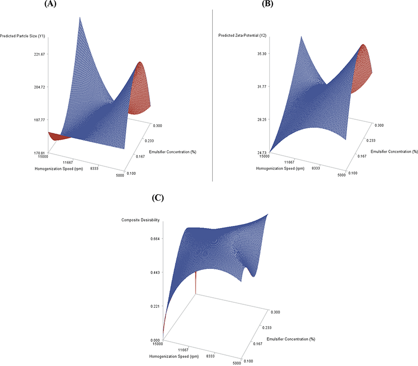
Each of the three-dimensional (3D) response surface plots was drawn with the vertical axis representing the predicted response and two horizontal axes indicating the two explanatory factors. Fig. 1A and 1B are the 3D response surface plots for the effects of the two actual factors on the two predicted responses.

Fig. 1. 3D surface plots of predicted responses and the composite desirability function. (A) 3D surface plot of the predicted response Y₁, (B) 3D surface plot of the predicted response Y₂, (C) 3D surface plot of the composite desirability function.

Download Original Figure

Multi-response optimization of two responses

In Ahn et al. (2017), the optimization objective was to minimize Y₁ (particle size) and maximize Y₂ (zeta-potential) simultaneously. For this multi-response optimization, we modified the desirability function technique of Derringer and Suich (1980). In this modified technique, first, we define the desirability function for the minimization of Y₁ as

D 1 = [Maximum(Y^1) − Y^1]/[Maximum(Y^1) − Minimum(Y^1)],

and define the desirability function for the maximization of Y₁ as

D 2 = [Maximum(Y^2) − Y^2]/[Maximum(Y^2) − Minimum(Y^2)] .

Here, for $Y^1$ , when $Y^1$ is minimized, D₁ becomes 1; otherwise 0≦D₁<1, and for $Y^2$ , when $Y^2$ is maximized, D₂ becomes 1; otherwise 0≦D₂<1. Now, we define CD, which means the composite desirability, as

CD = (D 1 D 2) (1/2)

which is the geometric mean of D₁ and D_2. Then, we find the combination of the values of X₁ and X₂ that maximizes CD. This combination is the optimum point of (X₁, X₂). Now, by converting this optimum point to the combination of the levels of the actual factors, we achieve the multi-response optimization of minimizing Y₁ and maximizing Y₂ simultaneously.

For the minimization and maximization of Y₁ and Y₂ and the maximization of CD, we performed the searches on a grid (Oh et al., 1995). First, we obtained Minimum ( $Y^1$ )=170.8131135, Maximum ( $Y^1$ )=221.6698750, Minimum ( $Y^2$ )=24.7334750, and Maximum ( $Y^2$ )=35.2957228, and using these values, we implemented our modified desirability function technique that maximizes the composite desirability defined above. Fig. 1C shows the 3D surface plot of the composite desirability function for our multi-response optimization. Table 2C presents the results of our multi-response optimization.

In Ahn et al. (2017), at their optimum point, their Y₁ value was 190.1 and their Y₂ value was −25.94±0.06, whereas, at our predicted optimum point, the predicted Y₁ was 183.4 and the predicted Y₂ was 30.93. We can see that our predicted minimum of Y₁ is smaller than their observed Y₁, and our predicted maximum of Y₂ is greater than their observed Y₂. Their optimum conditions for their multi-response optimization were F₁=speed of primary homogenization (rpm)=5,000 and F₂=concentration of emulsifier (%)=0.2071, whereas our optimum conditions are F₁=5,000 and F₂=0.295. We can see that our predicted combination of optimum factor levels is different from theirs. A validation experiment will be needed to verify the result of multi-response optimization obtained by the method proposed in this article.

Conclusion

This article suggests the use of the heterogeneous third-order model for better modeling and a modified desirability function technique for multi-response optimization. The heterogeneous third-order model can be used when (1) the experimental design is a two-factor central composite design having −1, 0, and 1 as the coded levels of factors, and (2) a second-order model fails to provide a good fit for the data. How to construct the heterogeneous third-order model is to use X₁, X₂, X₁², X₂², X₁X₂, X₁²X₂, and X₁X₂² as model terms. A modified desirability function technique first defines a desirability function for each response according to each optimization objective, and then finds out the combination of factor levels that maximizes the geometric mean of the values from desirability functions for multiple responses. An illustrative new analysis of the data from a previous research has produced statistical models with better fits and optimization results with better predictions. This suggestion is expected to help enhance the quality of response surface analyses of the experiments in food science of animal resources.

Notes

Conflict of Interest

The authors declare no potential conflict of interest.

Acknowledgments

This work was financially supported by the Graduate School of Public Administration at Korea University in 2018. And also this work was supported by the Basic Science Research Program through the National Research Foundation of Korea (NRF) funded by the Minister of Education, Science, and Technology (NRF-2016R1A2B4007519).

Notes

Author Contributions

Conceptualization: Rheem S, Rheem I, Oh S. Data curation: Rheem S. Formal analysis: Rheem S. Methodology: Rheem S, Rheem I, Oh S. Software: Rheem S. Investigation: Rheem S, Rheem I, Oh S. Writing - original draft: Rheem D, Oh S. Writing - review & editing: Rheem S, Rheem I, Oh S.

Notes

Ethics Approval

This article does not require IRB/IACUC approval because there are no human and animal participants.

References

Ahn SI, Park JH, Kim JH, Oh DG, Kim M, Chung D, Jhoo JW, Kim GY. 2017; Optimization of manufacturing conditions for improving storage stability of coffee-supplemented milk beverage using response surface methodology. Korean J Food Sci Anim Resour. 37:87-97

Box GEP, Wilson KB. 1951; On the experimental attainment of optimum conditions. J Royal Stat Soc Series B Methodol. 13:1-45

Derringer G, Suich R. 1980; Simultaneous optimization of several response variables. J Qual Technol. 12:214-219

Giunta AA. 1997 Aircraft multidisciplinary design optimization using design of experiments theory and response surface modeling methods. Ph.D. DissertationVirginia Polytechnic Institute and State University. Blacksburg, VA, USA: .

Myers RH, Montgomery DC, Anderson-Cook CM. 2009 Response surface methodology: Process and product optimization using designed experiments. 3^rd edJohn Wiley & Sons. Hoboken, NJ, USA: .

Oh S, Rheem S, Sim J, Kim S, Baek Y. 1995; Optimizing conditions for the growth of Lactobacillus casei YIT 9018 in tryptone-yeast extract-glucose medium by using response surface methodology. Appl Environ Microbiol. 61:3809-3814.

Rheem I, Rheem S. 2012; Response surface analysis in the presence of the lack of fit of the second-order polynomial regression model. J Korean Data Anal Soc. 14:2995-3001.

Rheem S, Oh S. 2019; Improving the quality of response surface analysis of an experiment for coffee-supplemented milk beverage: Data screening at the center point and maximum possible R-square. Food Sci Anim Resour. 39:114-120

SAS. 2013 SAS/GRAPH User’s Guide. Release 6.04. SAS Institute, Inc. Cary, NC, USA: .

10.

SAS. 2013 SAS/STAT User’s Guide. Release 6.04. SAS Institute, Inc. Cary, NC, USA: .

Related Articles

Improving the Quality of Response Surface Analysis of an Experiment for Coffee-supplemented Milk Beverage: II. Heterogeneous Third-order Models and Multi-response Optimization

Abstract

Introduction

Materials and Methods

Results and Discussion

Conclusion

Notes

Acknowledgments

Notes

Notes

References